


Here, I discuss a project in which I normalised Sample Superstore's CSV and then denormalised it into a star schema, using dbt and Snowflake.
I started modelling in PostgreSQL, which quickly began to feel limiting for what I wanted to do. I wanted to build a basic yet modern analytics engineering workflow, making use of cloud data warehousing, modularised SQL, version control and reproducible pipelines.
The aim was to learn how and why the same source data can and should be modelled differently depending on the use case.
In particular, I wanted to better understand two ideas:
- 1. OLTP-like normalised modelling
- 2. OLAP-like fact/dimensional modelling
Why Snowflake and dbt?
Snowflake and dbt overcame many limitations that I found when just using PostgreSQL.
Snowflake
Snowflake gave the project a cloud warehouse, rather than a database running locally on my device. Data teams usually do not build reports from local databases on a person's machine.
For the project, the raw Superstore CSV was loaded into Snowflake as a table. The table then became the starting point for the dbt-portion of the project.
dbt
PostgreSQL let me write SQL and store data, but the workflow relied on separate scripts, manual execution ordering, hard-coded table names and DDL (data definition language).
In dbt, each SQL script is a model. dbt can build all the models with a single command, in the correct order, based on the dependencies between them and without having to manually write any DDL. Models can reference one another by name, meaning that schema and table names do not need to be assigned in the warehouse beforehand.
Project-level configurations live in YAML, .yml, files. This allows for project-wide decisions to be made once, in one place, including which schema to build model layers into or deciding whether a model layer should be built as a set of tables or views.
Project Overview
The project has four transformation layers: raw, staging, intermediate and marts.
The raw layer contains the original Sample Superstore flat file. I manually loaded the CSV into Snowflake as a table. The raw Snowflake table was referenced within dbt using source().
The staging layer was the first wholly dbt layer. A staging layer's general purpose is to clean up raw data, i.e. by renaming columns or changing datatypes, making the source easier to work with.
The intermediate layer is where most of the modelling happened. The staging model was split into separate entities such as products, categories, customers, locations, dates, order items. The intermediate models reference the staging model using ref(), telling dbt that the intermediate models depend on the staging model, and allowing it to refer to the output of the staging layer by name.
The marts layer is the final, analytics-ready layer. The normalised, intermediate tables were partly denormalised and reshaped into a star schema.
Normalisation, denormalisation, OLTP and OLAP
The original flat file has a lot of repeat information. The same product name, segment, customer name, segment, etc., repeats across many rows.
Normalisation is the process of organising data into separate tables, representing entities, to reduce data duplication and improve consistency. Instead of storing all information in one big table, repeated entities are separated and connected through keys.
A primary key uniquely identifies a row in a table. A foreign key points to the primary key of another table. If a product belongs to a sub-category, the product table can store sub_category_id as a foreign key, which would point to the primary key in the sub-category table.
This avoids needing to store the same descriptive information repeatedly. Rather than storing category_name on every row, a normalised model can store all category names once in a category table, and then reference them through keys.
This sort of modelling is associated with OLTP (Online Transaction Processing) systems. OLTP systems form the backbone of day-to-day processes that allow businesses to function, like recording transactions as soon as they happen. They are designed to support accurate inserts, updates and deletes.
When modelling in an OLTP-way, questions like the following ought to be asked:
- How can repeated data be reduced?
- What separate entity types exist?
- How can they be related to one another?
In contrast, OLAP (Online Analytical Processing) systems are designed for analysis and reporting. The stress is not on accurate and efficient write queries, but on easy-to-use and quick read queries. Star and snowflake schemas are dimensional modelling structures commonly used in OLAP systems. My project partly denormalises the intermediate/normalised layer in order to make the tables more conducive to analytics.
When modelling in an OLAP-way, questions like these should be asked:
- What are we measuring?
- What (dimensions) do we want to analyse it by?
To illustrate why denormalisation is preferred for OLAP, let's answer the same question using both the intermediate (normalised) and marts (star schema): which customer bought the highest quantity of technology products in the West region?
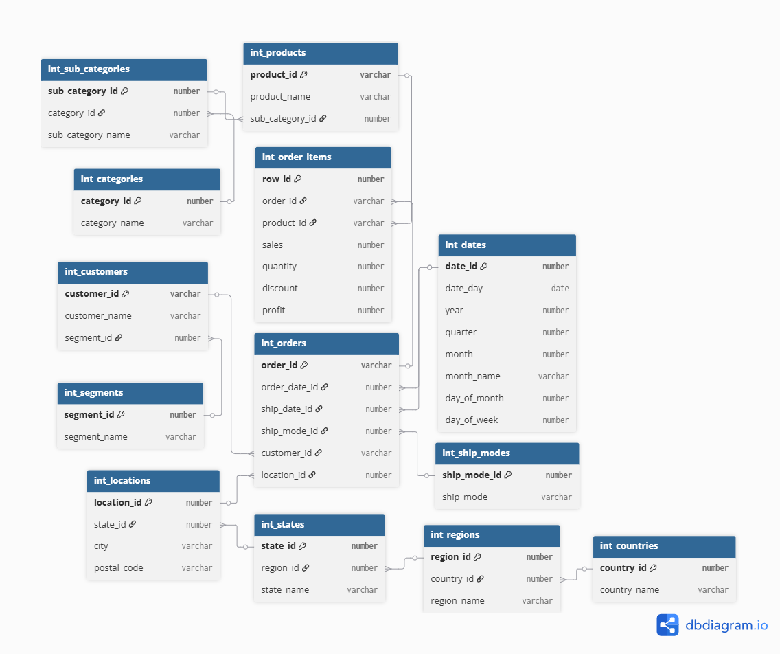
See below for more information on the tables for both layers and their schemas. Using the OLTP-like, normalised layer, the query is the following:
  SELECT
    c.customer_id,
    c.customer_name,
    r.region_name,
    cat.category_name,
    SUM(oi.quantity) AS total_quantity_bought,
    SUM(oi.sales) AS total_sales,
    SUM(oi.profit) AS total_profit

FROM SUPERSTORE_DB.DBT_SWADHIA_INTERMEDIATE.INT_ORDER_ITEMS AS oi

LEFT JOIN SUPERSTORE_DB.DBT_SWADHIA_INTERMEDIATE.INT_ORDERS AS o
    ON oi.order_id = o.order_id

LEFT JOIN SUPERSTORE_DB.DBT_SWADHIA_INTERMEDIATE.INT_CUSTOMERS AS c
    ON o.customer_id = c.customer_id

LEFT JOIN SUPERSTORE_DB.DBT_SWADHIA_INTERMEDIATE.INT_LOCATIONS AS l
    ON o.location_id = l.location_id

LEFT JOIN SUPERSTORE_DB.DBT_SWADHIA_INTERMEDIATE.INT_STATES AS st
    ON l.state_id = st.state_id

LEFT JOIN SUPERSTORE_DB.DBT_SWADHIA_INTERMEDIATE.INT_REGIONS AS r
    ON st.region_id = r.region_id

LEFT JOIN SUPERSTORE_DB.DBT_SWADHIA_INTERMEDIATE.INT_PRODUCTS AS p
    ON oi.product_id = p.product_id

LEFT JOIN SUPERSTORE_DB.DBT_SWADHIA_INTERMEDIATE.INT_SUB_CATEGORIES AS sc
    ON p.sub_category_id = sc.sub_category_id

LEFT JOIN SUPERSTORE_DB.DBT_SWADHIA_INTERMEDIATE.INT_CATEGORIES AS cat
    ON sc.category_id = cat.category_id

WHERE cat.category_name = 'Technology'
  AND r.region_name = 'West'

GROUP BY
    c.customer_id,
    c.customer_name,
    r.region_name,
    cat.category_name

ORDER BY
    total_quantity_bought DESC

LIMIT 1;
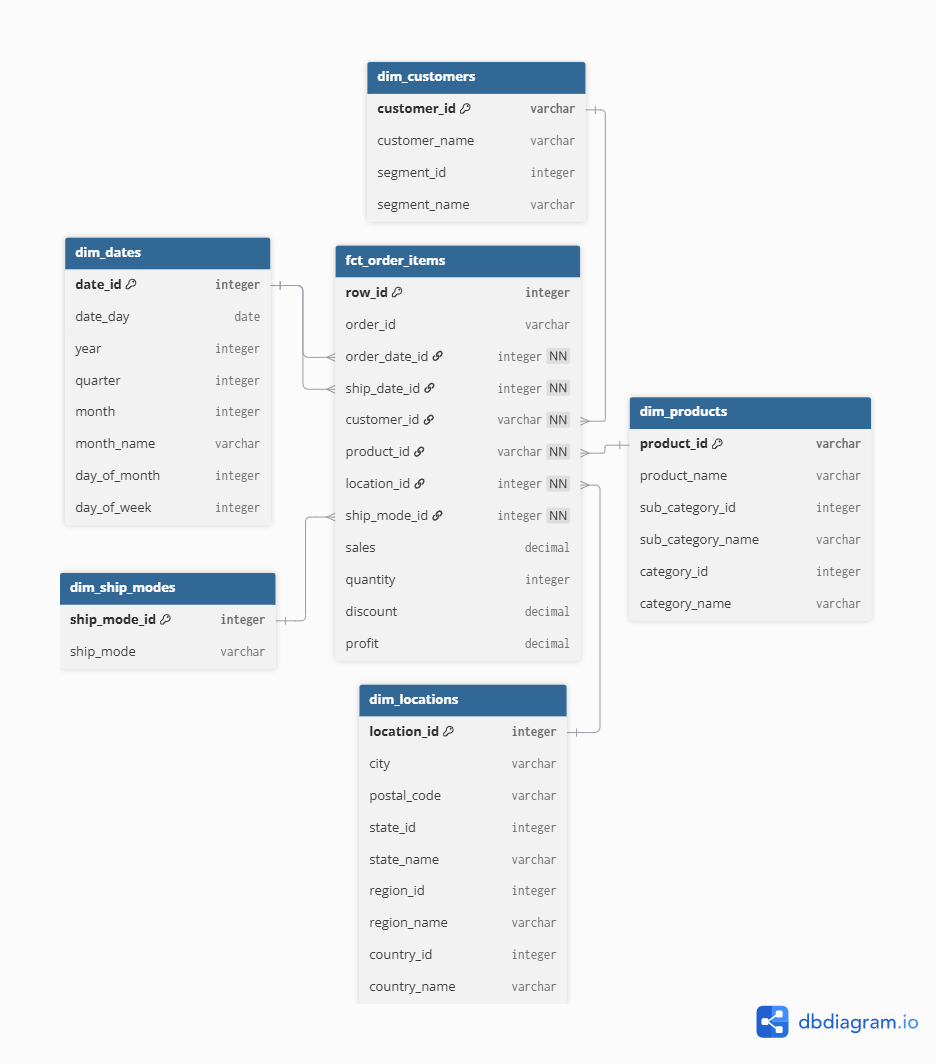
And for the OLAP-like, marts layer:
  SELECT
    c.customer_id,
    c.customer_name,
    l.region_name,
    p.category_name,
    SUM(f.quantity) AS total_quantity_bought,
    SUM(f.sales) AS total_sales,
    SUM(f.profit) AS total_profit

FROM SUPERSTORE_DB.DBT_SWADHIA_MARTS.FCT_ORDER_ITEMS AS f

LEFT JOIN SUPERSTORE_DB.DBT_SWADHIA_MARTS.DIM_CUSTOMERS AS c
    ON f.customer_id = c.customer_id

LEFT JOIN SUPERSTORE_DB.DBT_SWADHIA_MARTS.DIM_PRODUCTS AS p
    ON f.product_id = p.product_id

LEFT JOIN SUPERSTORE_DB.DBT_SWADHIA_MARTS.DIM_LOCATIONS AS l
    ON f.location_id = l.location_id

WHERE p.category_name = 'Technology'
  AND l.region_name = 'West'

GROUP BY
    c.customer_id,
    c.customer_name,
    l.region_name,
    p.category_name

ORDER BY
    total_quantity_bought DESC

LIMIT 1;
9 tables versus 4.
SQL queries against star schemas generally require fewer joins, are easier to understand, and are often better suited to analytical aggregations.
Building the Normalised Intermediate Layer
The granularity of the raw CSV is one row per order item.
See the schema below of the normalised layer. I discuss how I obtained the tables for the 'product hierarchy': categories, sub_categories, and products.
Starting with the categories table:
  select
    row_number() over (order by category_name) as category_id, -- index or primary key for categories
    category_name

from (
    select distinct
        trim(category) as category_name
    from {{ ref('stg_superstore') }}      -- reference to the output of another sql file, as opposed to hard-coded table
    where category is not null
)
Where the above code is from dbt and creates a row per category. Notice the FROM clause of the subquery:
from {{ ref('stg_superstore') }}
Which is a reference to a .sql file, or model with the name stg_superstore (the staging model). Tables and schemas do not need to be created beforehand and assigned a fixed name, when using dbt. Models reference the names of other models. The above query is materialising a view within Snowflake and yet notice the absence of DDL.
That query or model is named int_categories and is referenced in the model creating the normalised sub-categories table:
  with sub_categories as (

    select distinct
        trim(category) as category_name,
        trim(sub_category) as sub_category_name

    from {{ ref('stg_superstore') }}  -- reference to staging model

    where category is not null
      and sub_category is not null

),

categories as (

    select *
    from {{ ref('int_categories') }}   -- reference to int_categories model

)

select
    row_number() over (
        order by s.category_name, s.sub_category_name
    ) as sub_category_id,               -- primary key for sub-categories

    c.category_id,
    s.sub_category_name,
    s.category_name

from sub_categories as s

left join categories as c
    on s.category_name = c.category_name
This model, called int_sub_categories, extracts distinct sub-categories and links each one to its parent category. sub_category_id is the primary key of the sub-category table, and category_id is a foreign key pointing back to int_categories.
It gives a table like the following:
| sub_category_id | category_id | sub_category_name |
|---|---|---|
| 1 | 1 | Bookcases |
| 2 | 1 | Chairs |
| 3 | 1 | Furnishings |
| 4 | 2 | Appliances |
| 5 | 2 | Binders |
And the products model is defined as:
  select
    product_id,
    product_name,
    sub_category_id

from (
    select
        trim(product_id) as product_id,
        trim(product_name) as product_name,
        trim(category) as category_name,
        trim(sub_category) as sub_category_name,

        row_number() over (
            partition by trim(product_id)
            order by trim(product_name)
        ) as row_num

    from {{ ref('stg_superstore') }}

    where product_id is not null
) as p

left join {{ ref('int_sub_categories') }} as sc
    on p.sub_category_name = sc.sub_category_name

where row_num = 1;
Which gives a table like the following:
| product_id | product_name | sub_category_id |
|---|---|---|
| FUR-BO-10001798 | Bush Somerset Collection Bookcase | 1 |
| FUR-CH-10000454 | Hon Deluxe Fabric Upholstered Chair | 2 |
| OFF-BI-10003910 | DXL Angle-View Binders | 5 |
Measuring Redundancy Reduction
Normalisation reduces data redundancy. Repeated values are placed in separate tables and stored once.
To measure the reduction in redundancy, I compared the count of occurrences of an entity in the CSV to the number of rows in the corresponding normalised table. I only show a portion of the query due to its length:
  SELECT
    entity,
    flat_occurrences,
    normalised_rows,
    flat_occurrences - normalised_rows AS redundant_occurrences_removed,
    ROUND(
        100 * (flat_occurrences - normalised_rows)
        / NULLIF(flat_occurrences, 0),
        2
    ) AS redundancy_reduction_pct

FROM redundancy_metrics

ORDER BY
    redundancy_reduction_pct DESC;
The omitted portion of the query creates a CTE called redundancy_metrics, which calculates the number of occurrences of an entity in the flat file and compares this with the number of rows in the entity's normalised table. A series of unions stacks all values vertically. The query segment shown calculates the difference in an entity's occurrence within the CSV to its normalised table and expresses the difference as a percentage, giving this table:
| ENTITY | FLAT_OCCURRENCES | NORMALISED_ROWS | REDUNDANT_OCCURRENCES_REMOVED | REDUNDANCY_REDUCTION_PCT |
|---|---|---|---|---|
| countries | 9994 | 1 | 9993 | 99.99 |
| categories | 9994 | 3 | 9991 | 99.97 |
| segments | 9994 | 3 | 9991 | 99.97 |
| regions | 9994 | 4 | 9990 | 99.96 |
| ship_modes | 9994 | 4 | 9990 | 99.96 |
| sub_categories | 9994 | 17 | 9977 | 99.83 |
| states | 9994 | 49 | 9945 | 99.51 |
| locations | 9994 | 632 | 9362 | 93.68 |
| dates | 19988 | 1434 | 18554 | 92.83 |
| customers | 9994 | 793 | 9201 | 92.07 |
| products | 9994 | 1862 | 8132 | 81.37 |
| orders | 9994 | 5009 | 4985 | 49.88 |
Building the Star Schema
Again, a normalised schema is not conducive to analytics. To answer a simple question like, 'What were the total sales by category?,' would require joining order items to products, products to sub-categories and sub-categories to categories.
The marts layer of the project makes answering questions like this easier by partly denormalising the intermediate layer to create a star schema, with a central fact table surrounded by dimension tables.
As examples, I show how I obtained the products dimension table and the central fact table. Starting with products:
  select
    p.product_id,
    p.product_name,

    sc.sub_category_id,
    sc.sub_category_name,

    c.category_id,
    c.category_name

from {{ ref('int_products') }} as p

left join {{ ref('int_sub_categories') }} as sc
    on p.sub_category_id = sc.sub_category_id

left join {{ ref('int_categories') }} as c
    on sc.category_id = c.category_id
Wherein all three intermediate 'product hierarchy,' normalised tables have been referenced. This gives analysts one product dimension containing product, sub-category and category information. Instead of joining to three tables, they only need to join to dim_products.
And the fact table is given by:
  select
    oi.row_id,

    o.order_id,
    o.order_date_id,
    o.ship_date_id,

    o.customer_id,
    o.location_id,
    o.ship_mode_id,

    oi.product_id,

    oi.sales,
    oi.quantity,
    oi.discount,
    oi.profit

from {{ ref('int_order_items') }} as oi

left join {{ ref('int_orders') }} as o
    on oi.order_id = o.order_id
Validating the Transformations
There would have been no point in normalising and then denormalising if the transformations modified values. I used several queries to verify that the transformations did not change the underlying totals, one of which follows:
  WITH staging_totals AS (

    SELECT
        COUNT(*) AS row_count,
        SUM(sales) AS total_sales,
        SUM(profit) AS total_profit,
        SUM(quantity) AS total_quantity,
        SUM(discount) AS total_discount

    FROM SUPERSTORE_DB.DBT_SWADHIA_STAGING.STG_SUPERSTORE
),

fact_totals AS (

    SELECT
        COUNT(*) AS row_count,
        SUM(sales) AS total_sales,
        SUM(profit) AS total_profit,
        SUM(quantity) AS total_quantity,
        SUM(discount) AS total_discount

    FROM SUPERSTORE_DB.DBT_SWADHIA_MARTS.FCT_ORDER_ITEMS
)

SELECT
    'Row count' AS metric,
    s.row_count AS staging_value,
    f.row_count AS fact_value,
    s.row_count - f.row_count AS difference

FROM staging_totals AS s
CROSS JOIN fact_totals AS f

UNION ALL

SELECT
    'Total sales',
    s.total_sales,
    f.total_sales,
    s.total_sales - f.total_sales

FROM staging_totals AS s
CROSS JOIN fact_totals AS f

UNION ALL

SELECT
    'Total profit',
    s.total_profit,
    f.total_profit,
    s.total_profit - f.total_profit

FROM staging_totals AS s
CROSS JOIN fact_totals AS f

UNION ALL

SELECT
    'Total quantity',
    s.total_quantity,
    f.total_quantity,
    s.total_quantity - f.total_quantity

FROM staging_totals AS s
CROSS JOIN fact_totals AS f

UNION ALL

SELECT
    'Total discount',
    s.total_discount,
    f.total_discount,
    s.total_discount - f.total_discount

FROM staging_totals AS s
CROSS JOIN fact_totals AS f;
Which yields the following:
| METRIC | STAGING_VALUE | FACT_VALUE | DIFFERENCE |
|---|---|---|---|
| Row count | 9994.0000 | 9994.0000 | 0.0000 |
| Total sales | 2297200.8603 | 2297200.8603 | 0.0000 |
| Total profit | 286397.0217 | 286397.0217 | 0.0000 |
| Total quantity | 37873.0000 | 37873.0000 | 0.0000 |
| Total discount | 1561.0900 | 1561.0900 | 0.0000 |
Which shows that no differences have been introduced between the staging and marts layer.
Conclusion
The same CSV was modelled in two different ways to serve different purposes. The normalised layer broke apart the flat file into separate entities, thereby reducing redundancy. The star schema, instead, prioritised easier-to-write queries.
The validation queries showed that the change of structure did not change the underlying values.
The project remains basic. Next steps include adding tests and documentation, connecting the marts layer to a BI tool, and exploring whether an MCP layer could make the model queryable through natural language.