Explaining with: Data Normalization and Percentile calculations in Tableau & Power BI

Data analysis takes many shapes and forms, from simply getting to the answer quickly to interrogating details or small nuisances in the data. One way to investigate the data is to carry out comparison between different data points to see what or who performs best.

Obviously, it's hard to say what makes something the best and in the end it's a judgement we, as humans, will make. There are however, data analytics methods such as normalization, that allow us to provide additional views of the data to support our judgement.

So, in this blog, part of the Explaining with series, I will go over two different methods of data normalization; Z-Scores and Percentile calculations.

This blog is split up into four section:

1. What are Z-Scores and Percentiles, walking through a few examples using sports data (New Zeeland Rugby League player statistics).
2. How to carry out these calculations in Tableau.
3. How to carry out these calculations in Power BI.
4. Example visualisations showcasing these calculations.

Enjoy!

1. What are Z-Scores and Percentiles?

I'll try to showcase what both metrics are with sketches and data examples without going into too much detail.

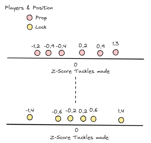
Let's say we have two groups of players, Props and Locks, and we record how many tackles they make in a game (how many times they stopped an opponent with the ball).

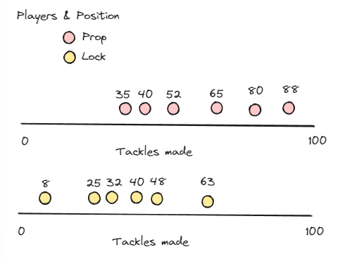
We can clearly see that both groups have different values associated with them. It would be unfair to make a direct comparison between the two groups, as it's likely that each of the groups have different opportunities to tackle during a game. So which of the two is a better performer within its own group? The 88 of the Props or the 63 of the Locks?

This is where Z-Scores can help us out;

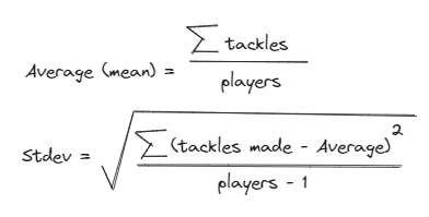
Z-Score looks at a sample set of data (in this case, Props and Locks are considered a group each), figures out what the average (mean) is within the set of data and how big the spread is (standard deviation).

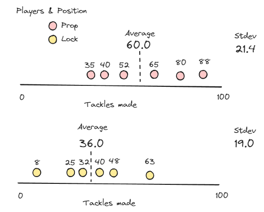
Each player within the set of data is than compared vs. those two metrics to see how far away they are from the average, e.g., seeing how much of an outlier they are. This is a form of normalization that allows us to compare players in different positions to one another.

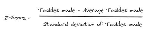
If we take the 88 from the Props and calculate their Z-Score we get (88-60)/21.4 = 1.3

For the Lock making 63 tackles we get (63-36)/19= 1.4

This shows that the Lock is more of an outlier (1.4 standard deviations away from the mean) then the Prop!

To give you an idea what it looks like if we plot all those players again, but than using the Z-Score of the Tackles made as an axis , we see that we have applied a baseline (the mean) so we can compare players between the groups more easily.

The second approach is using ranked percentiles, not to be confused with definitions as the 25th, 50th, etc percentile of a dataset (commonly determined for boxplots).

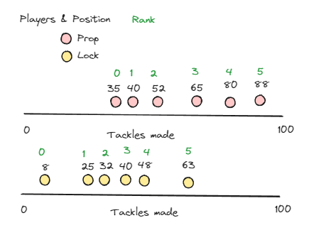
For the ranked percentiles we rank all players between 0 and 100. 0 being worst and 100 being best in the example of Tackles made.

This implies that, regardless of the dataset, there will always be an equal range of values for Ranked Percentiles, 0-100 (% or th Rank Percentile), whereas in Z-Scores the range van vary.

Let us walk through the same sample data of Props and Locks again. We start with assigning Ranks to each player with the group in ascending order starting at Rank 0.

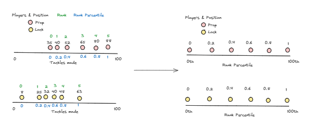
The Ranked Percentile can be calculated from those ranks using the following equation.

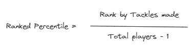
This now provides us with a Rank Percentile that allows us to pick the top, bottom and any in between players.

This makes it easier to pick out the top N players within a position and compare their metrics vs. other top N's. But we do loose the angle of what the metric is completely.

However, a combination of Tackles, Z-Scores of Tackles and Percentile Ranks of Tackles can work hand in hand to do some great player analysis!

A final note on how Rank Percentile deals with equal values; it skips a rank (values: 8,10,10,12 - rank: 0,2,2,3).

Have a look at a blog of our Data School Alumni; Lemis Tufail, who explains this using an example in Tableau.
https://www.thedataschool.co.uk/lemis-tufail/rank-percentile-on-tableau/

2. How to in Tableau

In Tableau we will utilize the table calculations to make sure our Z-Scores and Rank Percentiles are calculated dynamically based on filters applied and the desired aggregated metric.

I will walk through the calculated fields and table calculation setups for tackles per game. All other metrics follow the same logic.

As a reminder, the data is obtained from the New Zeeland Rugby League (NRL) website. https://www.nrl.com/

One row of data in the player stats table consists of one player and the game they played in. Metrics such as tackles made, meters run, etc are used to subsequently calculate the numbers we're interested in.

Take, tackles per game, which is defined as the SUM of Tackles made over the Distinct count of Games played. As there was no game id present, I created a unique identifier based on the round and year of the season.

tackles per game
SUM([Tackles Made])/COUNTD([Round by Year Sort])

This calculated field allows us to return each individual player name by position onto a scatter plot and adds up their total tackles made in all games over the total games they played in.

Furthermore, as this is aggregated on the sheet, we can use filters like; minutes played (row level information for how long they played in a game) on whether or not we want that row of data to be included or not.

But I digress, let's move onto the Z-Scores for tackles per game.

Our average (mean) is defined by a window_average of all players by their position, and our standard deviation (stdev) can be calculated using the window_stdev function.

z-score tackles per game
([tackles per game]-WINDOW_AVG([tackles per game]))
/
WINDOW_STDEV([tackles per game])

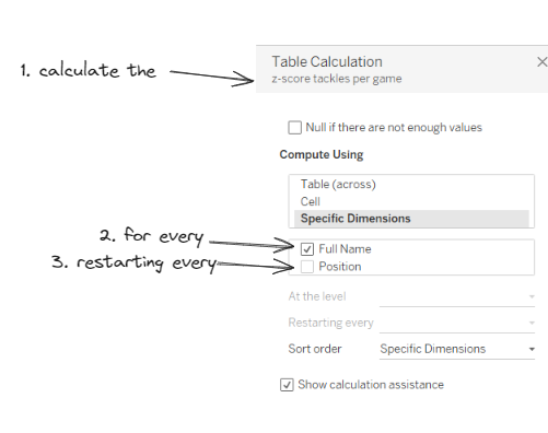
For the Table Calculation itself, we want both Full Name (player name) and Position on the marks card.

This way we can setup the table calculation by editing the table calculation and making sure Full Name is ticked and Position is unticked.

They way I like to phrase it is as follows:

Calculate the Z-Score for tackles per game for every Player , restarting the calculation every Position. The 'restarting every' refers to both the window_avg and window_stdev, hence, it will recalculate the averages and standard deviations for every different Position first. Afterwards, it takes the tackles per game for each player, subtract the average for their Position and divide the result by the standard deviation of the Position to get the Z-Score.

If both Full Name and Position were ticked, it would consider all players to be part of the same group and only calculate the window_average and window_stdev once, taking all marks into account. See below short video showcasing the differences.

For the Rank Percentile we utilize the rank_percentile function and combine it with the same tackles per game calculation we made prior. We can multiply it by 100 and add a "th" suffix if, format it as a % or leave it as a decimal place number. This depends on your preference.

percentile tackles made
RANK_PERCENTILE([tackles per game])*100

Follow the same guidelines for the Table Calculation setup as for Z-Scores to obtain the Rank Percentiles!

3. How to in Power BI

In Power BI we will utilize iterator functions (AverageX, RankX and StdevX.S) to make sure our Z-Scores and Rank Percentiles are calculated dynamically based on filters applied and the desired aggregated metric whilst maintaining the lowest level of granularity (one row equals one players' statistics of one match)

This does mean that some of these calculations are heavy on compute and expect some load times when applying filters and slicers. It can be significantly sped up by not using the iterator functions. You can replace them with normal functions (Average, Rank and Stdev.S) and pre-aggregating the tables. This would mean your averages, ranks, and standard deviations aren't re-calculated dynamically.

I will walk through the calculated measures and columns below.

As a reminder, the data is obtained from the New Zeeland Rugby League (NRL) website. https://www.nrl.com/

One row of data in the player stats table consists of one player and the game they played in. Metrics such as tackles made, meters run, etc are used to subsequently calculate the numbers we're interested in.

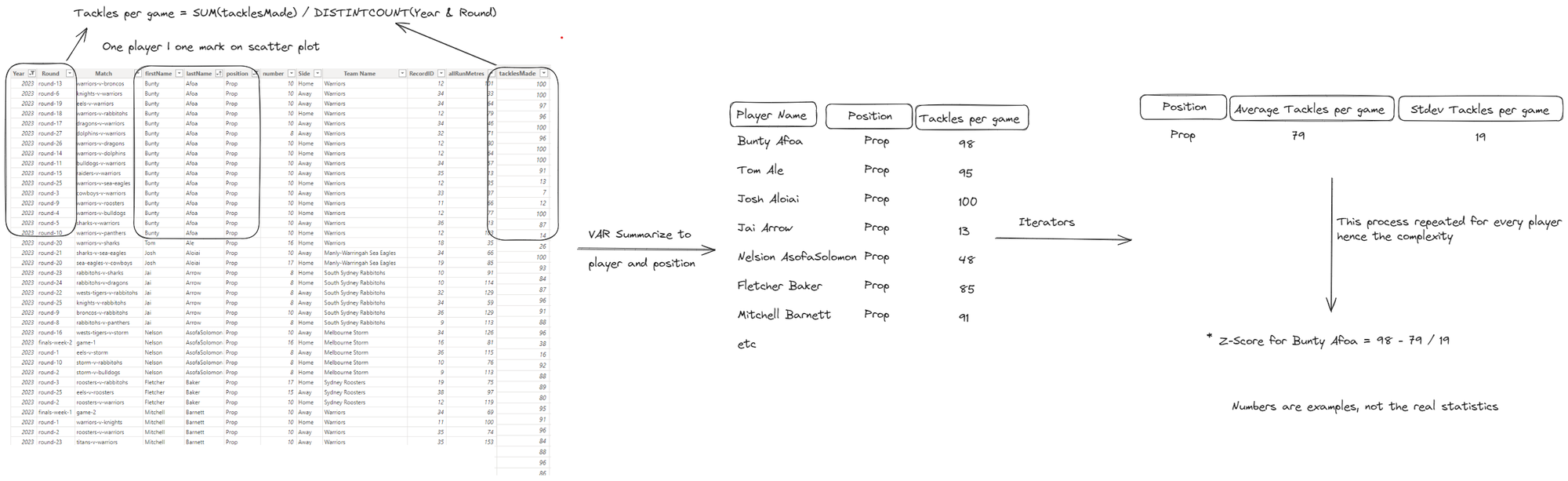
Take, tackles per game. This is defined as the SUM of tackles made divided by the total games played (as there is no game id, I've created a unique field that combines the round played and year of competition).

tackles per game = 
SUM('AllPlayerStats_2024-04-04 16_40_49'[tacklesMade])
/
DISTINCTCOUNT('AllPlayerStats_2024-04-04 16_40_49'[Round by Year Sort])

The Z-Score calculated measures are broken down into three parts:

1. For every point on the scatter plot, we need to know the average across the player and position. However, average needs to be carried out after aggregating the tackles per game to the player and position level first, before averaging out the resulting values. We achieve this with the summarize and filter function.
2. We then carry out the iterator functions over the newly created table and measure tacklespergame to obtain the correct averages and standard deviations.
3. we use the previously created tackles per game measure together with the average and standard deviation to obtain the Z-Score.

z-score tackles per game = 

VAR PlayerTacklesperGame = 
SUMMARIZE(
    FILTER(
            ALLSELECTED('AllPlayerStats_2024-04-04 16_40_49')
            ,'AllPlayerStats_2024-04-04 16_40_49'[position]=MAX('AllPlayerStats_2024-04-04 16_40_49'[position])
    )
    ,'AllPlayerStats_2024-04-04 16_40_49'[position]
    ,'AllPlayerStats_2024-04-04 16_40_49'[player name]
    ,"TacklesperGame",SUM('AllPlayerStats_2024-04-04 16_40_49'[tacklesMade])/DISTINCTCOUNT('AllPlayerStats_2024-04-04 16_40_49'[Round by Year Sort])
)

VAR AvgTacklesperGameperPosition = 
AVERAGEX(
    PlayerTacklesperGame
    ,[TacklesperGame]
)

VAR StdevTacklesperGameperPosition = 
STDEVX.S(
    PlayerTacklesperGame
    ,[TacklesperGame]
)

RETURN

([tackles per game] - AvgTacklesperGameperPosition)
/
StdevTacklesperGameperPosition

This also highlights the compute required for this calculation. the variable, VAR PlayerTacklesperGame, creates a table for every mark/circle on our scatter plot. This is required however, as we need to be able to see all other players values in order to return the averages and standard deviations by position!

As it's definitely not immediately evident what is happening in these calculations, I've tried to illustrate it with a schematic below.

The Rank Percentile calculations are also broken down into three parts:

1. Calculate the rank of a player based on their tackles per game.
2. Calculate the distinct players per position.
3. Combine the above in the Rank Percentile calculation as outlined earlier in part 1 of the blog to match the equation.

First the rank is calculated using the RankX() function. This returns the rank at the aggregated level of player and position.

player rank by position for tackles per game = 
VAR TacklesperGame = 
SUMMARIZE(
    FILTER(
            ALLSELECTED('AllPlayerStats_2024-04-04 16_40_49')
            ,'AllPlayerStats_2024-04-04 16_40_49'[position]=MAX('AllPlayerStats_2024-04-04 16_40_49'[position])
    )
    ,'AllPlayerStats_2024-04-04 16_40_49'[position]
    ,'AllPlayerStats_2024-04-04 16_40_49'[player name]
)

RETURN
RANKX(
    TacklesperGame
    ,[tackles per game]
    ,
    ,ASC
    ,Skip
)

We carry out a similar calculation we used in the Z-Score in order to obtain the distinct amount of players per position (available for every mark on the scatter plot).

Distinct Players per Position = 

VAR PlayersperPosition = 
SUMMARIZE(
    FILTER(
            ALLSELECTED('AllPlayerStats_2024-04-04 16_40_49')
            ,'AllPlayerStats_2024-04-04 16_40_49'[position]=MAX('AllPlayerStats_2024-04-04 16_40_49'[position])
    )
    ,'AllPlayerStats_2024-04-04 16_40_49'[position]
    ,"DistinctCount",DISTINCTCOUNT('AllPlayerStats_2024-04-04 16_40_49'[player name])
)

RETURN
MINX(PlayersperPosition, [DistinctCount])

To finalize the Rank Percentile we have to subtract 1 from the Rank (as we want to Rank starting from 0 and our RankX() starts at 1) and divide it by the total players -1.

percentile tackles per game per position = 
([player rank by position for tackles per game]-1) 
/ 
([Distinct Players per Position]-1)

And there we go, both Z-Scores and Rank Percentile calculations done in Power BI which can dynamically updated based on all our slicers, filters and parameters!

4. Visualisations

Below you'll find the visualisations I've put together to try and explain and showcase the use of these calculations. Both the Tableau packaged workbook and Power BI Report are available directly from the Explaining with GitHub Page.

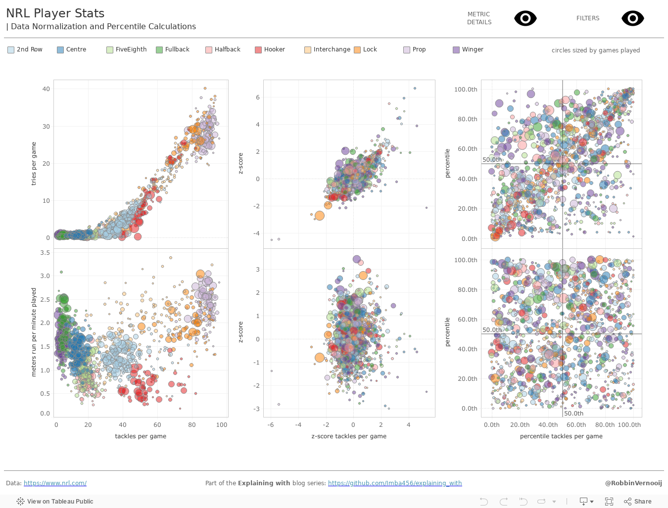
As per usual, feel free to reach out via social media if you have any questions!