


This blog will go through some of the best practice techniques when building a visualisation. Going over colour and chart choices as well as underlying data.
Colour blindness
The first viz best practice is one that is an accessibility feature for those with colour blindness. Red and green are common colours used in interface design; and due to how much it is used throughout society, most people are comfortable using it. The two colours have strong symbolic associations: with red representing a warning or to stop and green the opposite. These two colours being used are not a problem for most people, however there are a segment of people who suffer from red/green colour blindness. This would mean that using these colours in a dashboard would represent very little meaning for them and they would therefore gain less insights. 1 in 12 men and 1 in 200 women suffer from red/green colour blindness, so it is important to understand that the use of red and green – although generally effective – may not be best practice.
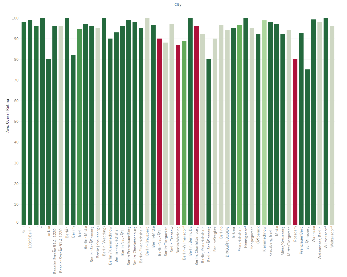
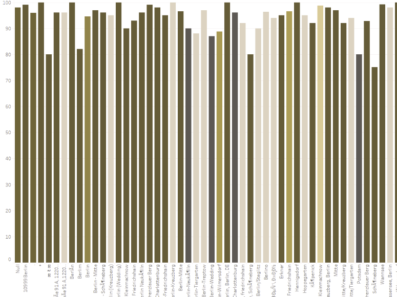
The two charts above show the what the use of red and green would look like; first to someone without colour blindness, and second to someone with colour blindness.
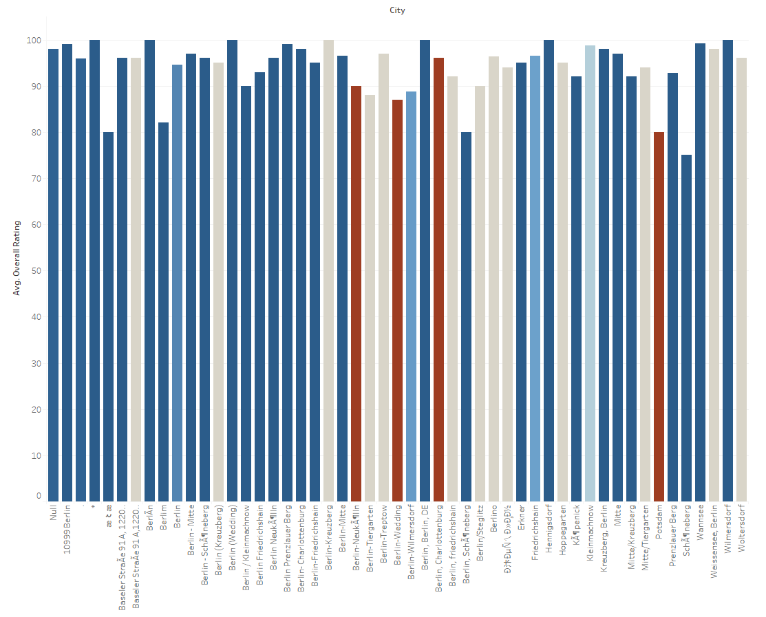
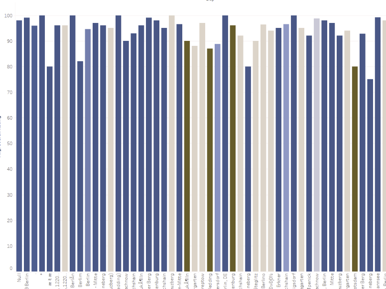
As shown by the two charts above, using alternative colours can be just at useful in allowing one to observe and gain insights. Using alternative colours like orange and blue can still get your message across, as well as be accessible to those with red/green colour-blindness. With the orange and blue chart we can still differentiate between the two distinct colours in the colour blind view.
Chart choices
A good chart choice can be the difference between the viewer comfortably gaining useful insights or being overwhelmed and confused. It can be tempting to use advance chart types but this can result in an adverse effect.
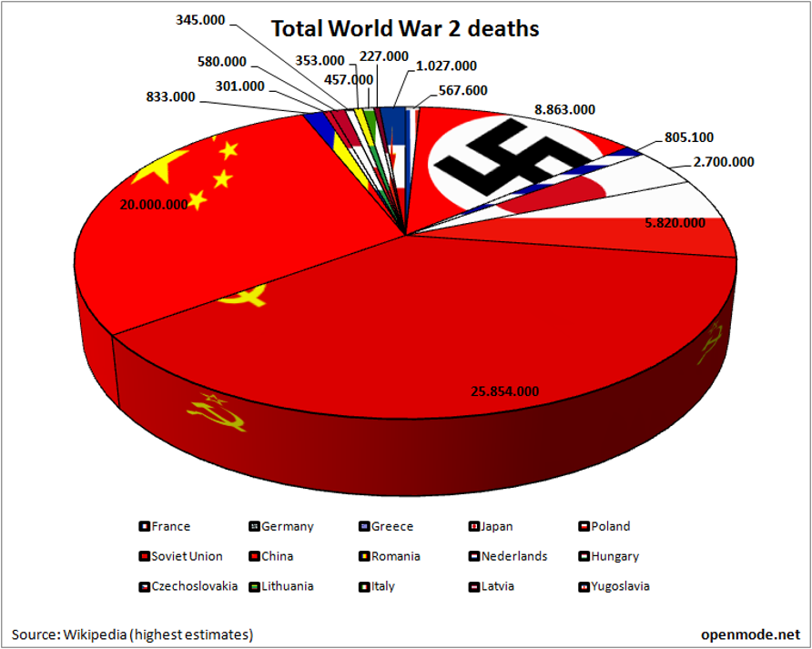
This is a 3d pie chart showing the total deaths in each country during world war 2. Although the 3d effect may look cool, this would not be a chart that would represent viz best practice.
The first problem is the 3d effect messes with the perspective. Any of the segments facing towards the front are overrepresented. This means the USSR deaths actually look proportionally larger. Removing the 3d effect still reveals some problems with this chart type. Where there are too many segments, it can be hard to assess the angles of each segment accurately. Having said that, pie charts can be useful for visualizing percentage of a total.
Another problem with this chart is the use of colour. Currently the segments are coloured by the flag that it represents. This becomes a problem when the flag colours are too similar. In this case there are multiple segments that use the colour red which makes it more difficult to differentiate.
The legend is also not good enough. It is too small, which means the flags are not visible in the legend. This isn’t helped with the large borders which restricts the view of the flags in the legend even further.
The final thing to note is the labelling. Every segment is labelled with the number of deaths that each of them represent. A chart should help remove numbers and make the data easier to view. The numbers remove the need for the pie and a table would have possibly been more useful.
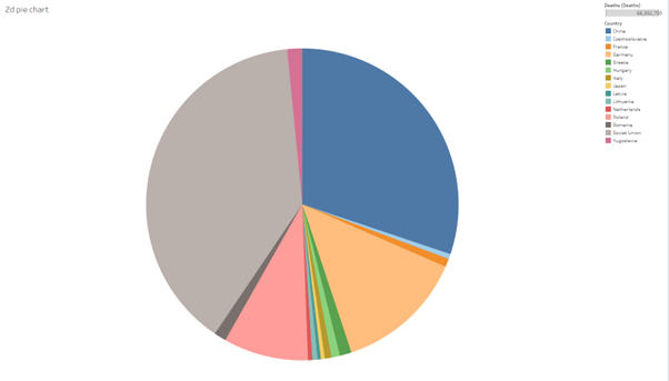
Changing the 3d pie to 2d represents a better chart type as no segment is overrepresented due to the perspective. The colours have also been adjusted so that each segment can be clearly defined.
As mentioned previously, although this is an improvement over the last chart it may not represent the best chart choice. This is due to segments being hard to compare, with proportional differences being hard to find.
We can take this chart a step further by making it a bar chart:
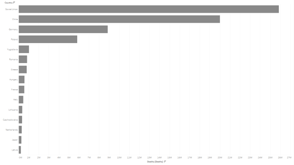
The bar chart displays all the information needed in a simple and clear manner. Adding mark labels can make this chart even easier to read. Proportions are all relative so it is easier to compare each country effectively. Moving to a bar chart also removes the need for coloured segments. This means that the bars can be coloured using another metric. This would mean you could extract more information from a bar chart than any of the two variations of pie chart shown.
Maps
Using maps to visualise data by geographic location in something that is commonly done. However it is important to ensure that any maps used provide an accurate representation of the data. It is a common mistake for many maps to just be population maps. There is less information about the data, and more information about where people live.
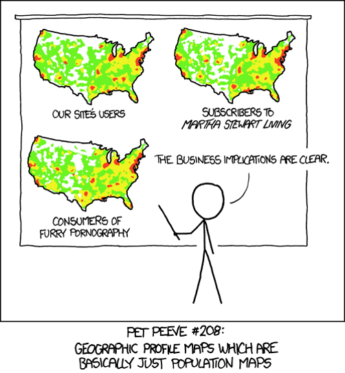
Due to this, maps can often not be the best way to show geographic data and can provide inaccurate insights if not understood properly.
A possible solution to this issue is by including the population in the analysis of the data. This can be done by converting the metric to a unit per capita. This should remove the impact of population on the data visualised on the map.
Underlying Data
Summary statistics are often used to visualise a larger set of data to a level of detail that is required. Often this can be useful, however there are times where summary statistics can ignore big differences.
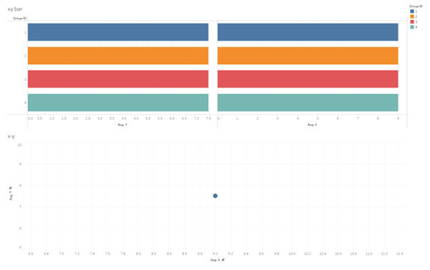
This dataset has two fields (x and y), and there are 4 groups (1,2,3 and 4). When using summary statistics, we find that the average of the two fields for the 4 groups is basically the same. The bar charts are the same length, with the scatterplot showing all 4 points overlayed at the same point. Just looking at the graph above it is very tempting to say that there is no real difference between the 4 groups. However, if we delve deeper into the data we can see how this statement is not accurate.
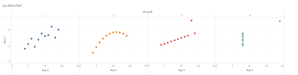
This is Anscombe’s quartet. It contains the same summary statistics, but with different distributions in the underlying data. Each of the 4 groups points are distributed differently and so have formed different shapes.
It is important to understand the underlaying data and when showing the average, it may also be useful to visualise the data in another way.
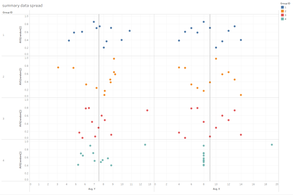
This is another example of how to visualise this summary data. Once again we can see how the distribution of the 4 groups varies.
Looks over Practicality
Often we can fall into the trap of creating visualisations that look really cool but have very little insights into the data and often creating them is not worth the squeeze. It is important to understand what insights need to be taken from the data and then make the best choice of chart to clearly depict this.
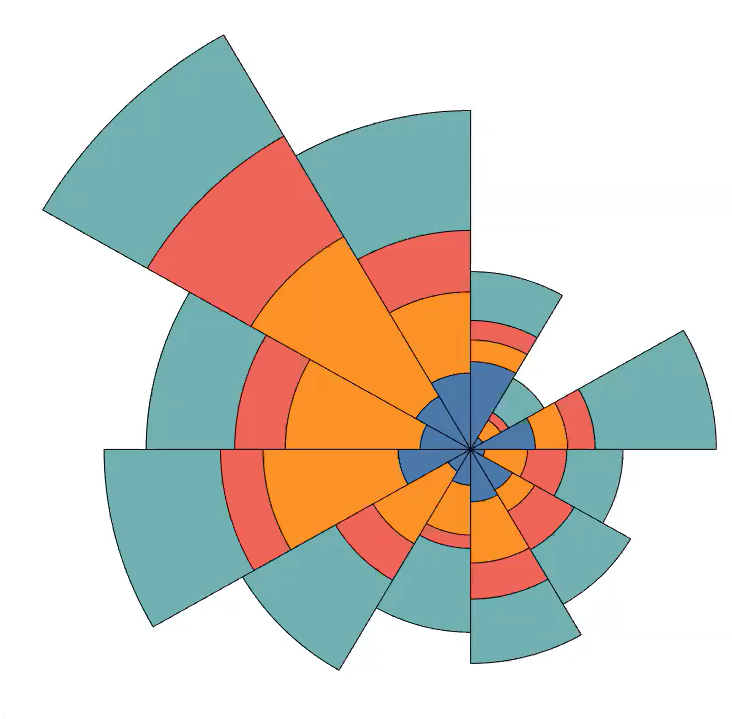
The coxcomb chart is a good example of this. It is a modified pie chart where each slice represents another interval or group. It looks very fancy, but is very difficult to make on tableau. It takes around 9 different calculations to create and the result is a chart that is difficult to read. Some insights can be drawn from this however it isn’t very clear and there are just better alternatives to this.
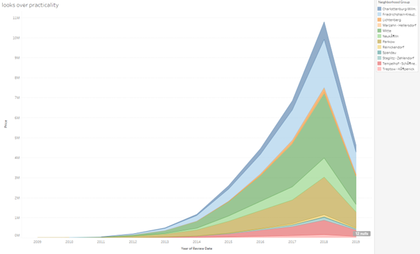
This is an area chart. Generally, it is pretty easy to read depending on what information you are trying to get out of it. For example, if you want to work out the proportional total of each category, this is an ideal choice. However, it is difficult to compare the individual categories and another chart would be required to allow for these insights.
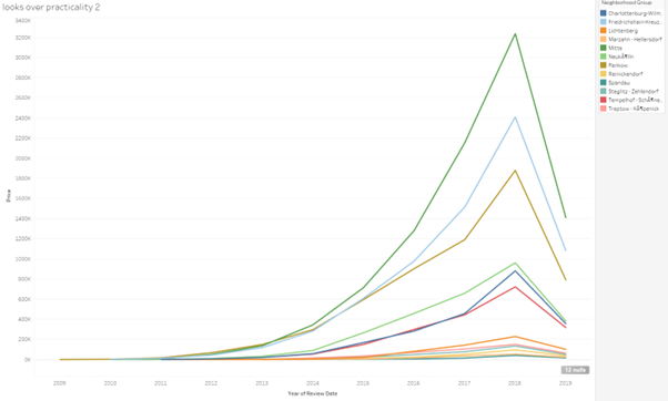
Another way of visualising the data is by using a line chart. Line charts are pretty easy to read, and you can gain some valuable insights. One being able to compare each category, which couldn’t be done on the area chart. However, there is no way to observe the total like the area chart.
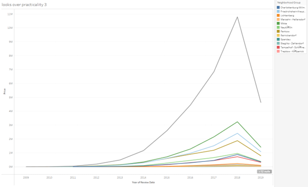
By adding a total line to the line graph by using a dual axis we can now see the total, much like the area chart. However, unlike the area chart there is no way to see the proportion of the total each category has. With the line graph with the addition of the total line we can compare categories as well as see the total.